Linear Algebra for Machine Learning: A Quick and Easy Beginners Guide
A brief guide on the fundamentals of linear algebra to get you started on your machine learning journey!
This article aims to give a brief introduction to the basics of linear algebra for machine learning, while also skipping the mathematical jargon and formalities that you may find unnecessary for machine learning engineers. Here you will find fundamentals like the basic definitions of vectors and matrices, as well as operations for them, and even some applications!
For those that are true beginners, I strongly encourage you to do exercises on everything explained here, and look up the concepts in more detail. This way you will reinforce what you have learned and won’t just forget it immediately after you finish reading this article. On the other hand if you just need a refresher, then I recommend you give the article a quick skim and pause where needed, as everything explained here is pretty basic. Now with that said, let’s get started.

1. What is Linear Algebra
Linear algebra as a whole is the study of linear functions and combinations, and extends further to the subject of abstract algebra, although in the context of linear algebra for machine learning you will mostly just see vectors and matrices. You can think of a vector as a finite list of numbers (or infinite, but you won’t need to consider that case here), and a matrix as multiple vectors stacked on top of one another. In a programming context, you can also think of lists and/or arrays as vectors and matrices.
2. Why Learn Linear Algebra
Linear algebra is a crucial part of many subject areas, like engineering, physics, and of course machine learning. We use it to turn informational data into a data type that we can perform mathematical and statistical operations on, and then convert it back afterwards to get new and predictive information. For examples of where you will use linear algebra, check out the second last section of this article.
Some more complicated fields, like the aforementioned field of physics, as well as robotics, makes use of a combination of linear algebra and calculus, which is commonly seen in the subject of multivariable calculus. Robotics is also a natural next step for many curious machine learning enthusiasts, so if you wish to pursue that field then grasping the fundamentals of linear algebra for machine learning should be of high importance to you.
3. Vectors
Formally, a vector is a finite set of elements where each element belongs to a field, and the vector itself follows various different axioms that always hold true.
But luckily, when learning linear algebra for machine learning specifically, you don’t need to know any of this mathematical jargon. All you really need to know is that a vector is a list of numbers, and that we can add and multiply vectors in a natural intuitive way.
Let’s start with an example of a vector, which we will call v:
As you can see, a vector is typically written as a sequence of numbers inside angled brackets. Vectors can be any length, and will often be written with variables inside them instead of numbers, for example:
4. Matrices
Now let’s introduce matrices, before getting into addition and multiplication. Since we are skipping mathematical formalities, you can think of a matrix as multiple vectors stacked on top of one another. We denote the dimension of a matrix as , where is the number of rows (or vectors stacked on top of one another), and is the number of columns (or the length of the vectors that are stacked). Note also that usually instead of angled brackets matrices will have either square or curved brackets. Consider the example below as a generalized matrix.
For generalized matrices, we need two indices to indicate the position of the elements, the first subscript indicating which row the element belongs to, and the other indicating the columns. Note the matrix need not have the same number of columns and rows. Here is an example of that:
5. Addition
Vector Addition
Adding vectors occurs in a natural and intuitive way. Consider the vectors:
Then when we add and together we add the components together to get another vector, where the component refers to the index (or subscript in this case) of an element in the vector. So .
Let’s do an example. Let’s give values to the vectors above so that they become:
Then
Matrix Addition
Matrix addition works the exact same way, so consider the following two matrices:
Then computing will give:
And that’s it for addition. Subtraction works in the same way except you replace all the additions with subtractions. As an exercise, can you work through ? Check your answer afterwords:
Note that the dimensions of both the vectors and matrices must be the same in order to add or subtract them.
6. Multiplication
Scalar Multiplication
Now onto multiplication. There are three types of multiplication, the first being scalar multiplication, which simply means multiplying a vector or matrix by a single value (i.e. scalar simply means singular value). For example, let your scalar variable be , and let
Then multiplying each by gives:
Indeed, multiplying both vectors and matrices by a scalar simply means to multiply each element inside them by that scalar. Now let us move on to the more complicated side of multiplication.
Dot Product
While not exactly a type of multiplication, the dot product is a very common operation performed on vectors that you must know, and will be needed in the next section. Luckily it is fairly simple, so consider two vectors again:
The dot product is then denoted by a thick dot, and will be computed by taking the products of the components of each vector and summing them up, i.e.
A notable fact about the dot product is that when it is zero, it means that the vectors are perpendicular. In a physical sense, thinking about two vectors that represent directions in the physical plane, this means that the angle between two vectors is 90 degrees. There is much more detail and meaning behind the dot product, but for now this is all you will need.
Vector and Matrix Multiplication
Although this might seem a bit odd, let’s start with matrix multiplication first. If you are multiplying two matrices, say and with size and respectively, then you must have that or else you cannot perform the multiplication. The resulting matrix will also be of dimension . This follows naturally by how it works, so let’s do an example by considering the following matrices:
Now think about each column or row of a matrix as a vector. Then in the resulting matrix the element in the row and column will be the dot product of the row vector in matrix and the column vector in matrix . So the result will look like:
While this may look complicated, remember each entry is just a scalar value, so if you had values to fill in for the variables you will end up with a more simple looking matrix like before. Also note for higher dimensional matrices the same formula is applied, but you will just have more tedious calculations to do, with a larger resulting matrix.
Now that you know matrix multiplication, seeing how vector multiplication is easy, because a vector is in fact just a matrix with dimension . This means that a vector is just a matrix with one row and columns. You can also look at a vector as a column vector with dimension , so it will have rows this time with only one column. Now multiplying a vector by a matrix is just like before, but here is an example anyways. Let . Then
As you can see this is a matrix of size , which can also be seen as a vector. Thus, you can use square or angled brackets here. It doesn’t really matter and in the common literature you may read the type of brackets for vector and matrix notation will often be used interchangeably.
The final thing to mention is something notable which is when you multiply a vector of with dimension by a vector of dimension , in which case the result of this operation will be a matrix of dimension . Consider the same above for example, with a column vector or matrix
Then
This operation in certain cases is called the outer product, and serves as the opposite of the dot product.
Cross Product
Although the cross product may not show up too often in the context of linear algebra for machine learning, it is a very common and important operation to know, and will surely come up at some point during your career. The cross product is just an operation on two 3 dimensional vectors, or equivalently vectors of length 3.
Consider the vectors from before,
then the cross product is denoted as
To get the values of and, , simply follow the following formula.
Since the cross product is an operation only in the 3-d plane, you can imagine it has real world implications, namely that it represents a vector that is perpendicular to both the vectors and . A couple facts about it that may come in handy: first is that if and are parallel to each other, then their cross product will be a vector of all zeroes. The second is that it is anti-commutative, meaning that . There is tons of more free information on the cross product that you can look up if need be, but in regards to linear algebra for machine learning, this should suffice for now.
7. Determinant
Another operation that doesn’t really resemble multiplication or any other typical operation is the determinant. While this may be a concept you won’t use too much in the context of linear algebra for machine learning, it is still a fundamental concept and also one that is necessary to understand invertible matrices (introduced in the next section).
You can think of the determinant as a function that returns a scalar value, given an input that is a square matrix. To calculate the determinant, we first need to look at it for a matrix:
The determinant is then calculated to be simply , and is commonly denoted by both and .
To see how this translates to larger matrices, let us extend this to a matrix:
Basically to compute we must break it down into smaller chunks, which is done by picking a row or column in the matrix, and then for each element of your chosen row or column, multiply it by the determinant of a matrix that is made up of elements that do not share the same row or columns as that element. Also, for the elements in your chosen row or column that had an even indexed position, multiply them by , and then sum all these products up to get your determinant.
Surely reading that for the first time sounds complicated, but it really isn’t once you see how it is done visually, so let’s calculate the determinant of . Note that when computing the determinant of a matrix, we often swap the square or curly brackets with the vertical lines or pipes as in the notation:
This process can naturally extend to larger matrices in a similar fashion, by continually breaking down the matrix in a recursive pattern. That being said, this level of understanding should suffice for now, and one of the most important facts regarding the determinant is its relation to other types of matrices, like invertible matrices, which we will move onto now.
8. Other Types of Matrices
There are other notable types of matrices that are important in the context of linear algebra for machine learning that can be obtained by performing some kind of operation or transformation to any matrix. The most important ones are listed here, and once you have a grasp for the basics of this linear algebra material, feel free to check out some of the other types of matrices.
Transpose
The first is the transpose of a matrix. To make the next concepts more clear, consider a dimensional matrix now:
Then the transpose of a matrix is obtained by swapping the off diagonal elements with each other. More formally, this means that we swap the elements with the elements. Take a look at transpose to see this more clearly, where we denote the transpose with a superscript .
This can also work for matrices that have dimension where and are not equal to each other. In this case the resulting matrix will have dimension . Consider the previous matrix A but with the third column removed, i.e.
Then
Furthermore, this extends to vectors as well since they are often seen as a one column or one row matrix. In fact, in a lot of math textbooks the standard way to write a vector will be as a row, like , and then when the author wants you to think of the vector as a column vector they will write it as its transpose:
Identity Matrix
Just a quick definition here, the identity matrix is something you must know and basically acts as the value in matrix multiplication, meaning that multiplying any matrix or vector by the identity matrix will result in the same matrix or vector you started with. It is defined as follows:
This of course scales to any dimension you wish, but note that it will always have the same number of rows and columns (a square matrix), and the diagonal elements will always be and everything else will be .
Invertible Matrix
Think about a number, say 5, then the inverse of 5 would be 1/5, and multiplying 5 by its inverse will give you 1. Well an invertible matrix is simply a matrix that has a similar inverse matrix like the 1 / 5, such that by multiplying the matrix by its inverse you will get the identity matrix.
Moreover, a matrix is categorically called an invertible matrix if and only if it indeed has such an inverse. The reason for stating this again is because it is not guaranteed that a matrix will have an inverse, and thus may not be an invertible matrix. So how do we know if a matrix is invertible? Well luckily you need only check two things. Firstly, the matrix must be a square, and secondly, the determinant of the matrix must be zero, which you already know how to do now. There is so much more to learn about invertible matrices, and they have many more uses in other fields. While it may not be necessary, I would recommend at some point reading up on invertible matrices a bit more.
9. Examples of Linear Algebra for Machine Learning
Now that we’ve covered all of the fundamentals of linear algebra for machine learning, let’s move on to the fun part, which is where and when we actually get to use this stuff. Well, below are just a few common examples, but do keep in mind learning about these applications in detail will be quite a challenge if you have not yet fully grasped the above material.
One-Hot Encoding
Sometimes in machine learning you will have data that may be troublesome to handle. One common way to deal with this is with one-hot encoding. Say you have multiple classes of objects, then you would label each class with a vector filled with all zeros except for one element, which will be a 1 in a unique spot/index in the vector relative to all other classes (note: this means that the dot product between any two of the one-hot encoded vectors will be zero).
Principal Component Analysis
A common concept in machine learning that you will learn early on is principal component analysis, or PCA for short. As its name suggests, the aim of PCA is to find variables that give the most amount of information, and then discard other variables that are more or less redundant. This way, you reduce the dimensionality of your problem, which essentially means it simplifies the problem.
The linear algebra used here can get a bit more complicated than what was given in this post, but the fundamentals explained above should enable you to understand any extra necessary material quickly. (Quick tip: read up on eigenvalue and eigenvectors before looking into PCA).
Neural Networks
Perhaps the most popular occurrence of the linear algebra for machine learning you learned here is in deep learning and neural networks. If you haven’t yet introduced yourself to neural networks, I encourage you to do so soon, as it is truly the hottest topic in all of machine learning and artificial intelligence. But once you do you will see that it is a collection of nodes and lines that connect them, and these lines have weights attached to them which will be stored inside a matrix. Computations performed when training a neural network will largely be matrix addition and multiplication, so honing in on your skills in linear algebra for machine learning in particular will come in handy.
Computer Vision
Computer vision is a branch of machine learning that typically deals with unstructured data in the form of images. In fact, an image is simply a matrix filled with values that describe the color of each pixel in the image, so naturally you can already see the material you learned in this linear algebra for machine learning article coming into play here. You then create predictive models using convolutional neural networks, which are a special type of neural network typically reserved for images.
In computer vision the output of your algorithm may be another image, like an altered version of your input image, or a word or number describing the original image, like a description of the type of animal in your input image. What you get out of you convolution neural networks really depends on the type of problem you have, but there are a wide variety of problems being solved with these methods, so definitely look into later if this sounds interesting.
Natural Language Processing
Natural language processing (NLP) is another branch of machine learning and typically deals with words as your input data. But how do we convert words into data that we can train predictive models on? Well you can use linear algebra of course, by changing each word into a vector using something called word embeddings. Similar to computer vision, which has its own special type of neural network, NLP problems tend to use its own special type of neural network, called recurrent neural networks. The details on how these work go pretty in-depth, so I’ll skip it here, but either way you can clearly see now how important it is to learn the necessary linear algebra for machine learning as it has so many uses in this field, so it’s never too early to start learning it!
10. Moving Forward
Now that you understand the basics of linear algebra for machine learning, you can go on to learn everything explained above in more detail and fill in any other gaps in your linear algebra knowledge that you may have. Again, this article was just meant to be an introduction to the fundamentals of linear algebra, so that you could get a feel for what it is like. I recommend doing exercises on the vector and matrix operations explained above, to reinforce your learnings. That way, you can come back to this article whenever you forget something, and remember it much faster.
As you saw, there are a ton of applications of linear algebra for machine learning, and there are many more that were not mentioned. But as you continue your machine learning and artificial intelligence journey, you will have the fundamentals of linear algebra to understand its use in any of those settings, and will soon see that it is used almost everywhere.
If you liked this article, there are many more types and applications of math in the field of machine learning and other fields. When you are ready I would recommend brushing up on your calculus or stats knowledge next, as those are just as fundamental to machine learning as linear algebra. And for the curious and ambitious who want to go the extra mile, I’d recommend looking into subjects like graph theory and even quantum computing, since those are exciting fields that are still somewhat related to machine learning.