Keras for Beginners: Implementing a Recurrent Neural Network
A beginner-friendly guide on using Keras to implement a simple Recurrent Neural Network (RNN) in Python.
![]()
Keras is a simple-to-use but powerful deep learning library for Python. In this post, we’ll build a simple Recurrent Neural Network (RNN) and train it to solve a real problem with Keras.
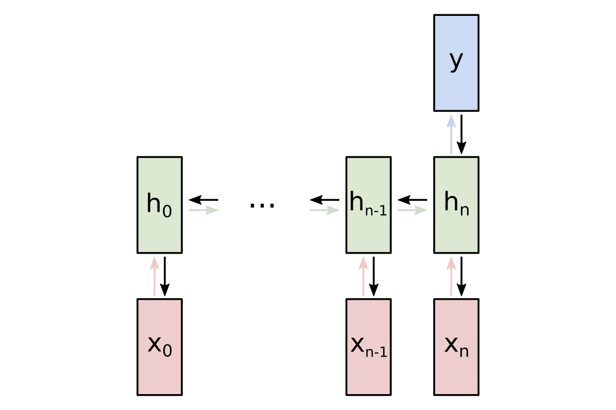
This post is intended for complete beginners to Keras but does assume a basic background knowledge of RNNs. My introduction to Recurrent Neural Networks covers everything you need to know (and more) for this post - read that first if necessary.
Here we go!
Just want the code? The full source code is at the end.
The Problem: Classifying Movie Reviews
We’re going to tackle a classic introductory Natural Language Processing (NLP) problem: doing sentiment analysis on IMDb movie reviews from Stanford AI Lab’s Large Movie Review Dataset.
Here are two samples from the dataset:
| Excerpt from review | Sentiment |
|---|---|
| Liked Stanley & Iris very much. Acting was very good. Story had a unique and interesting arrangement… | Positive 👍 |
| This is the worst thing the TMNT franchise has ever spawned. I was a kid when this came out and I still thought it was deuce… | Negative 👎 |
1. Setup
First, we need to download the dataset. You can either:
- download it from my site (I’ve hosted a copy with files we won’t need for this post removed), or
- download it from the official site.
Either way, you’ll end up with a directory with the following structure:
dataset/
  test/
    neg/
    pos/
  train/
    neg/
    pos/
Next, we’ll install dependencies. All we need is Tensorflow, which comes packaged with Keras as its official high-level API:
$ pip install tensorflow2. Preparing the Data
Tensorflow has a very easy way for us to read in our dataset: text_dataset_from_directory. Here’s how we’ll do it:
from tensorflow.keras.preprocessing import text_dataset_from_directory

# Assumes you're in the root level of the dataset directory.
# If you aren't, you'll need to change the relative paths here.
train_data = text_dataset_from_directory("./train")
test_data = text_dataset_from_directory("./test")
dataset is now a Tensorflow Dataset object we can use later!
There’s one more small thing to do. If you browse through the dataset, you’ll notice that some of the reviews include <br /> markers in them, which are HTML line breaks. We want to get rid of those, so we’ll modify our data prep a bit:
from tensorflow.keras.preprocessing import text_dataset_from_directory
from tensorflow.strings import regex_replace

def prepareData(dir):
  data = text_dataset_from_directory(dir)
  return data.map(
    lambda text, label: (regex_replace(text, '<br />', ' '), label),
  )

train_data = prepareData('./train')
test_data = prepareData('./test')
Now, all <br /> instances in our dataset have been replaced with spaces. You can try printing some of the dataset if you want:
for text_batch, label_batch in train_data.take(1):
  print(text_batch.numpy()[0])
  print(label_batch.numpy()[0]) # 0 = negative, 1 = positive
We’re ready to start building our RNN!
3. Building the Model
We’ll use the Sequential class, which represents a linear stack of layers. To start, we’ll instantiate an empty sequential model and define its input type:
from tensorflow.keras.models import Sequential
from tensorflow.keras import Input

model = Sequential()
model.add(Input(shape=(1,), dtype="string"))
Our model now takes in 1 string input - time to do something with that string.
3.1 Text Vectorization
Our first layer will be a TextVectorization layer, which will process the input string and turn it into a sequence of integers, each one representing a token.
from tensorflow.keras.layers.experimental.preprocessing import TextVectorization

max_tokens = 1000
max_len = 100
vectorize_layer = TextVectorization(
  # Max vocab size. Any words outside of the max_tokens most common ones
  # will be treated the same way: as "out of vocabulary" (OOV) tokens.
  max_tokens=max_tokens,
  # Output integer indices, one per string token
  output_mode="int",
  # Always pad or truncate to exactly this many tokens
  output_sequence_length=max_len,
)
To initialize the layer, we need to call .adapt():
# Call adapt(), which fits the TextVectorization layer to our text dataset.
# This is when the max_tokens most common words (i.e. the vocabulary) are selected.
train_texts = train_data.map(lambda text, label: text)
vectorize_layer.adapt(train_texts)
Finally, we can add the layer to our model:
model.add(vectorize_layer)3.2 Embedding
Our next layer will be an Embedding layer, which will turn the integers produced by the previous layer into fixed-length vectors.
from tensorflow.keras.layers import Embedding

# Previous layer: TextVectorization
max_tokens = 1000
# ...
model.add(vectorize_layer)

# Note that we're using max_tokens + 1 here, since there's an
# out-of-vocabulary (OOV) token that gets added to the vocab.
model.add(Embedding(max_tokens + 1, 128))
Reading more on popular word embeddings like GloVe or Word2Vec may help you understand what Embedding layers are and why we use them.
3.3 The Recurrent Layer
Finally, we’re ready for the recurrent layer that makes our network a RNN! We’ll use a Long Short-Term Memory (LSTM) layer, which is a popular choice for this kind of problem. It’s very simple to implement:
from tensorflow.keras.layers import LSTM

# 64 is the "units" parameter, which is the
# dimensionality of the output space.
model.add(LSTM(64))
To finish off our network, we’ll add a standard fully-connected (Dense) layer and an output layer with sigmoid activation:
from tensorflow.keras.layers import Dense

model.add(Dense(64, activation="relu"))
model.add(Dense(1, activation="sigmoid"))
The sigmoid activation outputs a number between 0 and 1, which is perfect for our problem - 0 represents a negative review, and 1 represents a positive one.
4. Compiling the Model
Before we can begin training, we need to configure the training process. We decide a few key factors during the compilation step, including:
- The optimizer. We’ll stick with a pretty good default: the Adam gradient-based optimizer. Keras has many other optimizers you can look into as well.
- The loss function. Since we only have 2 output classes (positive and negative), we’ll use the Binary Cross-Entropy loss. See all Keras losses.
- A list of metrics. Since this is a classification problem, we’ll just have Keras report on the accuracy metric.
Here’s what that compilation looks like:
model.compile(
  optimizer='adam',
  loss='binary_crossentropy',
  metrics=['accuracy'],
)
Onwards!
5. Training the Model
Training our model with Keras is super easy:
model.fit(train_data, epochs=10)Putting all the code we’ve written thus far together and running it gives us results like this:
Epoch 1/10
loss: 0.6441 - accuracy: 0.6281
Epoch 2/10
loss: 0.5544 - accuracy: 0.7250
Epoch 3/10
loss: 0.5670 - accuracy: 0.7200
Epoch 4/10
loss: 0.4505 - accuracy: 0.7919
Epoch 5/10
loss: 0.4221 - accuracy: 0.8062
Epoch 6/10
loss: 0.4051 - accuracy: 0.8156
Epoch 7/10
loss: 0.3870 - accuracy: 0.8247
Epoch 8/10
loss: 0.3694 - accuracy: 0.8339
Epoch 9/10
loss: 0.3530 - accuracy: 0.8406
Epoch 10/10
loss: 0.3365 - accuracy: 0.8502
We’ve achieved 85% train accuracy after 10 epochs! There’s certainly a lot of room to improve (this problem isn’t that easy), but it’s not bad for a first effort.
6. Using the Model
Now that we have a working, trained model, let’s put it to use. The first thing we’ll do is save it to disk so we can load it back up anytime:
model.save_weights('cnn.h5')We can now reload the trained model whenever we want by rebuilding it and loading in the saved weights:
model = Sequential()

# ... add the model's layers

# Load the model's saved weights.
model.load_weights('cnn.h5')
Using the trained model to make predictions is easy: we pass a string to predict() and it outputs a score.
# Should print a very high score like 0.98.
print(model.predict([
  "i loved it! highly recommend it to anyone and everyone looking for a great movie to watch.",
]))

# Should print a very low score like 0.01.
print(model.predict([
  "this was awful! i hated it so much, nobody should watch this. the acting was terrible, the music was terrible, overall it was just bad.",
]))
7. Extensions
There’s much more we can do to experiment with and improve our network. Some examples of modifications you could make to our CNN include:
Network Depth
What happens if we add Recurrent layers? How does that affect training and/or the model’s final performance?
model = Sequential()

# ...

# Return the full sequence instead of just the last
# output of the sequence.
model.add(LSTM(64, return_sequences=True))
# This second recurrent layer's input sequence is the
# output sequence of the previous layer.
model.add(LSTM(64))
Dropout
What if we incorporated dropout (e.g. via Dropout layers), which is commonly used to prevent overfitting?
from tensorflow.keras.layers import Dropout

model = Sequential()

# ...

# Examples of common ways to use dropout below. These
# parameters are not necessarily the most optimal.
model.add(LSTM(64, dropout=0.25, recurrent_dropout=0.25))
model.add(Dense(64, activation="relu"))
model.add(Dropout(0.5))
Text Vectorization Parameters
The max_tokens and max_len parameters used in our TextVectorization layer are natural candidates for tinkering:
- Too low of a
max_tokenswill exclude potentially useful words from our vocabulary, while too high of one may increase the complexity and training time of our model. - Too low of a
max_lenwill impact our model’s performance on longer reviews, while too high of one again may increase the complexity and training time of our model.
Pre-processing
All we did to clean our dataset was remove <br /> markers. There may be other pre-processing steps that would be useful to us. For example:
- Removing “useless” tokens (e.g. ones that are extremely common or otherwise not useful)
- Fixing common mispellings / abbreviations and standardizing slang
Conclusion
You’ve implemented your first RNN with Keras! I’ll include the full source code again below for your reference.
Further reading you might be interested in include:
- My Keras for Beginners series, which has more Keras guides.
- My complete beginner’s guide to understanding RNNs.
- The official getting started with Keras guide.
- More posts on Neural Networks or Keras.
Thanks for reading! The full source code is below.
The Full Code
# I'm importing everything up here to improve readability later on,
# but it's also common to just:
#     import tensorflow as tf
# and then access whatever you need directly from tf.
from tensorflow.keras.preprocessing import text_dataset_from_directory
from tensorflow.strings import regex_replace
from tensorflow.keras.layers.experimental.preprocessing import TextVectorization
from tensorflow.keras.models import Sequential
from tensorflow.keras import Input
from tensorflow.keras.layers import Dense, LSTM, Embedding, Dropout

def prepareData(dir):
  data = text_dataset_from_directory(dir)
  return data.map(
    lambda text, label: (regex_replace(text, '<br />', ' '), label),
  )

# Assumes you're in the root level of the dataset directory.
# If you aren't, you'll need to change the relative paths here.
train_data = prepareData('./train')
test_data = prepareData('./test')

for text_batch, label_batch in train_data.take(1):
  print(text_batch.numpy()[0])
  print(label_batch.numpy()[0]) # 0 = negative, 1 = positive


model = Sequential()

# ----- 1. INPUT
# We need this to use the TextVectorization layer next.
model.add(Input(shape=(1,), dtype="string"))

# ----- 2. TEXT VECTORIZATION
# This layer processes the input string and turns it into a sequence of
# max_len integers, each of which maps to a certain token.
max_tokens = 1000
max_len = 100
vectorize_layer = TextVectorization(
  # Max vocab size. Any words outside of the max_tokens most common ones
  # will be treated the same way: as "out of vocabulary" (OOV) tokens.
  max_tokens=max_tokens,
  # Output integer indices, one per string token
  output_mode="int",
  # Always pad or truncate to exactly this many tokens
  output_sequence_length=max_len,
)

# Call adapt(), which fits the TextVectorization layer to our text dataset.
# This is when the max_tokens most common words (i.e. the vocabulary) are selected.
train_texts = train_data.map(lambda text, label: text)
vectorize_layer.adapt(train_texts)

model.add(vectorize_layer)

# ----- 3. EMBEDDING
# This layer turns each integer (representing a token) from the previous layer
# an embedding. Note that we're using max_tokens + 1 here, since there's an
# out-of-vocabulary (OOV) token that gets added to the vocab.
model.add(Embedding(max_tokens + 1, 128))

# ----- 4. RECURRENT LAYER
model.add(LSTM(64))

# ----- 5. DENSE HIDDEN LAYER
model.add(Dense(64, activation="relu"))

# ----- 6. OUTPUT
model.add(Dense(1, activation="sigmoid"))


# Compile and train the model.
model.compile(loss="binary_crossentropy", optimizer="adam", metrics=["accuracy"])
model.fit(train_data, epochs=10)

model.save_weights('rnn')

model.load_weights('rnn')

# Try the model on our test dataset.
model.evaluate(test_data)

# Should print a very high score like 0.98.
print(model.predict([
  "i loved it! highly recommend it to anyone and everyone looking for a great movie to watch.",
]))

# Should print a very low score like 0.01.
print(model.predict([
  "this was awful! i hated it so much, nobody should watch this. the acting was terrible, the music was terrible, overall it was just bad.",
]))